Tabulate biomarker effects on survival by subgroup
Source:R/survival_biomarkers_subgroups.R
survival_biomarkers_subgroups.RdTabulate the estimated effects of multiple continuous biomarker variables across population subgroups.
Usage
tabulate_survival_biomarkers(
  df,
  vars = c("n_tot", "n_tot_events", "median", "hr", "ci", "pval"),
  groups_lists = list(),
  control = control_coxreg(),
  label_all = lifecycle::deprecated(),
  time_unit = NULL,
  na_str = default_na_str(),
  .indent_mods = 0L
)
Arguments
- df
(
data.frame)
containing all analysis variables, as returned byextract_survival_biomarkers().- vars
-
(
character)
the names of statistics to be reported among:n_tot_events: Total number of events per group.n_tot: Total number of observations per group.median: Median survival time.hr: Hazard ratio.ci: Confidence interval of hazard ratio.pval: p-value of the effect. Note, one of the statisticsn_totandn_tot_events, as well as bothhrandciare required.
- groups_lists
(named
listoflist)
optionally contains for eachsubgroupsvariable a list, which specifies the new group levels via the names and the levels that belong to it in the character vectors that are elements of the list.- control
(
list)
a list of parameters as returned by the helper functioncontrol_coxreg().- label_all
please assign thelabel_allparameter within theextract_survival_biomarkers()function when creatingdf.- time_unit
(
string)
label with unit of median survival time. DefaultNULLskips displaying unit.- na_str
(
string)
string used to replace allNAor empty values in the output.- .indent_mods
(named
integer)
indent modifiers for the labels. Defaults to 0, which corresponds to the unmodified default behavior. Can be negative.
Details
These functions create a layout starting from a data frame which contains the required statistics. The tables are then typically used as input for forest plots.
Functions
tabulate_survival_biomarkers(): Table-creating function which creates a table summarizing biomarker effects on survival by subgroup.
Note
In contrast to tabulate_survival_subgroups() this tabulation function does
not start from an input layout lyt. This is because internally the table is
created by combining multiple subtables.
See also
h_tab_surv_one_biomarker() which is used internally, extract_survival_biomarkers().
Examples
library(dplyr)

adtte <- tern_ex_adtte

# Save variable labels before data processing steps.
adtte_labels <- formatters::var_labels(adtte)

adtte_f <- adtte %>%
  filter(PARAMCD == "OS") %>%
  mutate(
    AVALU = as.character(AVALU),
    is_event = CNSR == 0
  )
labels <- c("AVALU" = adtte_labels[["AVALU"]], "is_event" = "Event Flag")
formatters::var_labels(adtte_f)[names(labels)] <- labels

# Typical analysis of two continuous biomarkers `BMRKR1` and `AGE`,
# in multiple regression models containing one covariate `RACE`,
# as well as one stratification variable `STRATA1`. The subgroups
# are defined by the levels of `BMRKR2`.

df <- extract_survival_biomarkers(
  variables = list(
    tte = "AVAL",
    is_event = "is_event",
    biomarkers = c("BMRKR1", "AGE"),
    strata = "STRATA1",
    covariates = "SEX",
    subgroups = "BMRKR2"
  ),
  label_all = "Total Patients",
  data = adtte_f
)
df
#>   biomarker              biomarker_label n_tot n_tot_events   median        hr
#> 1    BMRKR1 Continuous Level Biomarker 1   200          141 753.5176 1.0010939
#> 2       AGE                          Age   200          141 753.5176 1.0106406
#> 3    BMRKR1 Continuous Level Biomarker 1    70           52 735.4722 0.9905065
#> 4       AGE                          Age    70           52 735.4722 1.0106279
#> 5    BMRKR1 Continuous Level Biomarker 1    68           42 858.9952 0.9623210
#> 6       AGE                          Age    68           42 858.9952 1.0360765
#> 7    BMRKR1 Continuous Level Biomarker 1    62           47 727.8043 1.0770946
#> 8       AGE                          Age    62           47 727.8043 1.0009890
#>         lcl      ucl conf_level      pval     pval_label       subgroup    var
#> 1 0.9538978 1.050625       0.95 0.9646086 p-value (Wald) Total Patients    ALL
#> 2 0.9871004 1.034742       0.95 0.3787395 p-value (Wald) Total Patients    ALL
#> 3 0.9142220 1.073156       0.95 0.8155443 p-value (Wald)            LOW BMRKR2
#> 4 0.9621192 1.061582       0.95 0.6735773 p-value (Wald)            LOW BMRKR2
#> 5 0.8708694 1.063376       0.95 0.4509368 p-value (Wald)         MEDIUM BMRKR2
#> 6 0.9727439 1.103532       0.95 0.2707796 p-value (Wald)         MEDIUM BMRKR2
#> 7 0.9756250 1.189118       0.95 0.1412524 p-value (Wald)           HIGH BMRKR2
#> 8 0.9678535 1.035259       0.95 0.9541048 p-value (Wald)           HIGH BMRKR2
#>                      var_label row_type
#> 1               Total Patients  content
#> 2               Total Patients  content
#> 3 Continuous Level Biomarker 2 analysis
#> 4 Continuous Level Biomarker 2 analysis
#> 5 Continuous Level Biomarker 2 analysis
#> 6 Continuous Level Biomarker 2 analysis
#> 7 Continuous Level Biomarker 2 analysis
#> 8 Continuous Level Biomarker 2 analysis

# Here we group the levels of `BMRKR2` manually.
df_grouped <- extract_survival_biomarkers(
  variables = list(
    tte = "AVAL",
    is_event = "is_event",
    biomarkers = c("BMRKR1", "AGE"),
    strata = "STRATA1",
    covariates = "SEX",
    subgroups = "BMRKR2"
  ),
  data = adtte_f,
  groups_lists = list(
    BMRKR2 = list(
      "low" = "LOW",
      "low/medium" = c("LOW", "MEDIUM"),
      "low/medium/high" = c("LOW", "MEDIUM", "HIGH")
    )
  )
)
df_grouped
#>   biomarker              biomarker_label n_tot n_tot_events   median        hr
#> 1    BMRKR1 Continuous Level Biomarker 1   200          141 753.5176 1.0010939
#> 2       AGE                          Age   200          141 753.5176 1.0106406
#> 3    BMRKR1 Continuous Level Biomarker 1    70           52 735.4722 0.9905065
#> 4       AGE                          Age    70           52 735.4722 1.0106279
#> 5    BMRKR1 Continuous Level Biomarker 1   138           94 777.8929 0.9801709
#> 6       AGE                          Age   138           94 777.8929 1.0236283
#> 7    BMRKR1 Continuous Level Biomarker 1   200          141 753.5176 1.0010939
#> 8       AGE                          Age   200          141 753.5176 1.0106406
#>         lcl      ucl conf_level      pval     pval_label        subgroup    var
#> 1 0.9538978 1.050625       0.95 0.9646086 p-value (Wald)    All Patients    ALL
#> 2 0.9871004 1.034742       0.95 0.3787395 p-value (Wald)    All Patients    ALL
#> 3 0.9142220 1.073156       0.95 0.8155443 p-value (Wald)             low BMRKR2
#> 4 0.9621192 1.061582       0.95 0.6735773 p-value (Wald)             low BMRKR2
#> 5 0.9235465 1.040267       0.95 0.5094582 p-value (Wald)      low/medium BMRKR2
#> 6 0.9859367 1.062761       0.95 0.2224475 p-value (Wald)      low/medium BMRKR2
#> 7 0.9538978 1.050625       0.95 0.9646086 p-value (Wald) low/medium/high BMRKR2
#> 8 0.9871004 1.034742       0.95 0.3787395 p-value (Wald) low/medium/high BMRKR2
#>                      var_label row_type
#> 1                 All Patients  content
#> 2                 All Patients  content
#> 3 Continuous Level Biomarker 2 analysis
#> 4 Continuous Level Biomarker 2 analysis
#> 5 Continuous Level Biomarker 2 analysis
#> 6 Continuous Level Biomarker 2 analysis
#> 7 Continuous Level Biomarker 2 analysis
#> 8 Continuous Level Biomarker 2 analysis

## Table with default columns.
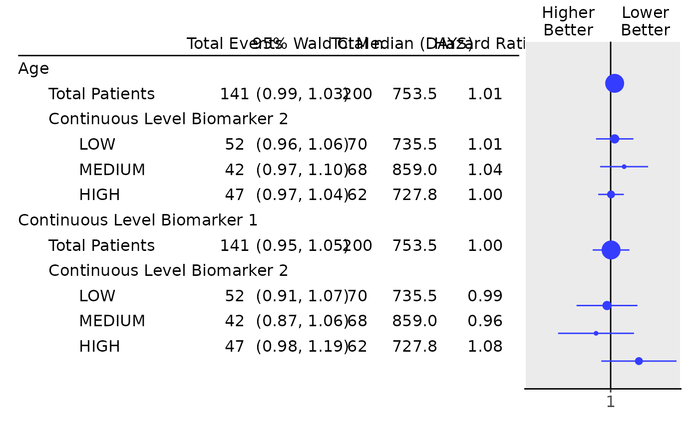
tabulate_survival_biomarkers(df)
#>                                  Total n   Total Events   Median   Hazard Ratio   95% Wald CI    p-value (Wald)
#> ———————————————————————————————————————————————————————————————————————————————————————————————————————————————
#> Age
#>   Total Patients                   200         141        753.5        1.01       (0.99, 1.03)       0.3787
#>   Continuous Level Biomarker 2
#>     LOW                            70           52        735.5        1.01       (0.96, 1.06)       0.6736
#>     MEDIUM                         68           42        859.0        1.04       (0.97, 1.10)       0.2708
#>     HIGH                           62           47        727.8        1.00       (0.97, 1.04)       0.9541
#> Continuous Level Biomarker 1
#>   Total Patients                   200         141        753.5        1.00       (0.95, 1.05)       0.9646
#>   Continuous Level Biomarker 2
#>     LOW                            70           52        735.5        0.99       (0.91, 1.07)       0.8155
#>     MEDIUM                         68           42        859.0        0.96       (0.87, 1.06)       0.4509
#>     HIGH                           62           47        727.8        1.08       (0.98, 1.19)       0.1413

## Table with a manually chosen set of columns: leave out "pval", reorder.
tab <- tabulate_survival_biomarkers(
  df = df,
  vars = c("n_tot_events", "ci", "n_tot", "median", "hr"),
  time_unit = as.character(adtte_f$AVALU[1])
)

## Finally produce the forest plot.
# \donttest{
g_forest(tab, xlim = c(0.8, 1.2))

# }
# }