![[Stable]](figures/lifecycle-stable.svg)
Fits a Cox regression model and estimate hazard ratio to describe the effect size in a survival analysis.
Usage
h_coxreg_univar_formulas(variables, interaction = FALSE)

h_coxreg_multivar_formula(variables)

fit_coxreg_univar(variables, data, at = list(), control = control_coxreg())

# S3 method for summary.coxph
tidy(x, ...)

h_coxreg_univar_extract(effect, covar, data, mod, control = control_coxreg())

# S3 method for coxreg.univar
tidy(x, ...)

fit_coxreg_multivar(variables, data, control = control_coxreg())

h_coxreg_multivar_extract(var, data, mod, control = control_coxreg())

# S3 method for coxreg.multivar
tidy(x, ...)

s_coxreg(df, .var)

summarize_coxreg(
  lyt,
  conf_level,
  multivar = FALSE,
  vars = c("n", "hr", "ci", "pval")
)
Arguments
- variables
(
list)
a named list corresponds to the names of variables found indata, passed as a named list and corresponding totime,event,arm,strata, andcovariatesterms. Ifarmis missing fromvariables, then only Cox model(s) including thecovariateswill be fitted and the corresponding effect estimates will be tabulated later.- interaction
(
flag)
ifTRUE, the model includes the interaction between the studied treatment and candidate covariate. Note that for univariate models without treatment arm, and multivariate models, no interaction can be used so that this needs to beFALSE.- data
(
data frame)
the dataset containing the variables to fit the models.- at
(
listofnumeric)
when the candidate covariate is anumeric, useatto specify the value of the covariate at which the effect should be estimated.- control
(
list)
a list of parameters as returned by the helper functioncontrol_coxreg().- x
(
list)
Result of the Cox regression model fitted byfit_coxreg_multivar().- ...
additional arguments for the lower level functions.
- effect
(
string)
the treatment variable.- covar
(
string)
the name of the covariate in the model.- mod
(
coxph)
Cox regression model fitted bysurvival::coxph().- df
(
data frame)
data set containing all analysis variables.- .var, var
(
string)
single variable name that is passed byrtableswhen requested by a statistics function.- lyt
(
layout)
input layout where analyses will be added to.- conf_level
(
proportion)
confidence level of the interval.- multivar
(
flag)
ifTRUE, the multi-variable Cox regression will run and no interaction will be considered between the studied treatment and c candidate covariate. Default isFALSEfor univariate Cox regression including an arm variable. When no arm variable is included in the univariate Cox regression, then alsoTRUEshould be used to tabulate the covariate effect estimates instead of the treatment arm effect estimate across models.- vars
(
character)
the name of statistics to be reported amongn(number of observation),hr(Hazard Ratio),ci(confidence interval),pval(p.value of the treatment effect) andpval_inter(the p.value of the interaction effect between the treatment and the covariate).
Value
The function h_coxreg_univar_formulas returns a character vector coercible
into formulas (e.g stats::as.formula()).
The function h_coxreg_univar_formulas returns a character vector coercible
into formulas (e.g stats::as.formula()).
The function fit_coxreg_univar returns a coxreg.univar class object which is a named list
with 5 elements:
mod: Cox regression models fitted bysurvival::coxph().data: The original data frame input.control: The original control input.vars: The variables used in the model.at: Value of the covariate at which the effect should be estimated.
The function fit_coxreg_multivar returns a coxreg.multivar class object which is a named list
with 4 elements:
mod: Cox regression model fitted bysurvival::coxph().data: The original data frame input.control: The original control input.vars: The variables used in the model.
Details
Cox models are the most commonly used methods to estimate the magnitude of the effect in survival analysis. It assumes proportional hazards: the ratio of the hazards between groups (e.g., two arms) is constant over time. This ratio is referred to as the "hazard ratio" (HR) and is one of the most commonly reported metrics to describe the effect size in survival analysis (NEST Team, 2020).
Functions
-
h_coxreg_univar_formulas(): Helper for Cox Regression FormulaCreates a list of formulas. It is used internally by
fit_coxreg_univar()for the comparison of univariate Cox regression models. -
h_coxreg_multivar_formula(): Helper for Multi-variable Cox Regression FormulaCreates a formulas string. It is used internally by
fit_coxreg_multivar()for the comparison of multi-variable Cox regression models. Interactions will not be included in multi-variable Cox regression model. fit_coxreg_univar(): Fit a series of univariate Cox regression models given the inputs.-
tidy(summary.coxph): Custom tidy method forsurvival::coxph()summary results.Tidy the
survival::coxph()results into adata.frameto extract model results. h_coxreg_univar_extract(): Utility function to help tabulate the result of a univariate Cox regression model.-
tidy(coxreg.univar): Custom tidy method for a Univariate Cox RegressionTidy up the result of a Cox regression model fitted by
fit_coxreg_univar(). fit_coxreg_multivar(): Fit a multi-variable Cox regression model.-
h_coxreg_multivar_extract(): Tabulation of Multi-variable Cox RegressionsUtility function to help tabulate the result of a multi-variable Cox regression model for a treatment/covariate variable.
-
tidy(coxreg.multivar): Custom tidy method for a Multi-variable Cox RegressionTidy up the result of a Cox regression model fitted by
fit_coxreg_multivar(). s_coxreg(): transforms the tabulated results fromfit_coxreg_univar()andfit_coxreg_multivar()into a list. Not much calculation is done here, it rather prepares the data to be used by the layout creating function.summarize_coxreg(): layout creating function.
Note
The usual formatting arguments for the layout creating function
summarize_coxreg are not yet accepted (.stats, .indent_mod, .formats,
.labels).
When using fit_coxreg_univar there should be two study arms.
Examples
# Testing dataset [survival::bladder].
library(survival)
library(rtables)
set.seed(1, kind = "Mersenne-Twister")
dta_bladder <- with(
data = bladder[bladder$enum < 5, ],
data.frame(
time = stop,
status = event,
armcd = as.factor(rx),
covar1 = as.factor(enum),
covar2 = factor(
sample(as.factor(enum)),
levels = 1:4, labels = c("F", "F", "M", "M")
)
)
)
labels <- c("armcd" = "ARM", "covar1" = "A Covariate Label", "covar2" = "Sex (F/M)")
formatters::var_labels(dta_bladder)[names(labels)] <- labels
dta_bladder$age <- sample(20:60, size = nrow(dta_bladder), replace = TRUE)
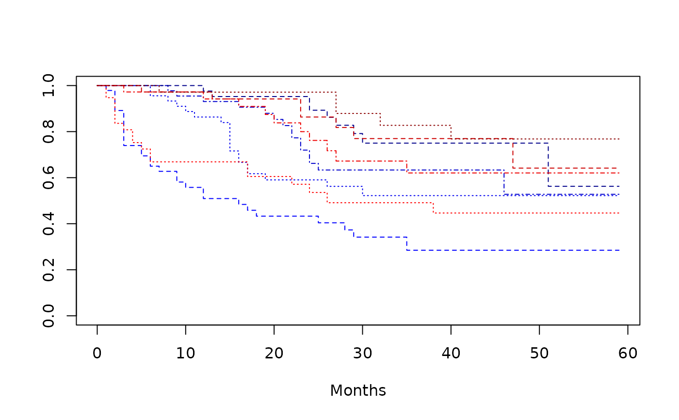
plot(
survfit(Surv(time, status) ~ armcd + covar1, data = dta_bladder),
lty = 2:4,
xlab = "Months",
col = c("blue1", "blue2", "blue3", "blue4", "red1", "red2", "red3", "red4")
)
 # `h_coxreg_univar_formulas`
## Simple formulas.
h_coxreg_univar_formulas(
variables = list(
time = "time", event = "status", arm = "armcd", covariates = c("X", "y")
)
)
#> ref
#> "survival::Surv(time, status) ~ armcd"
#> X
#> "survival::Surv(time, status) ~ armcd + X"
#> y
#> "survival::Surv(time, status) ~ armcd + y"
## Addition of an optional strata.
h_coxreg_univar_formulas(
variables = list(
time = "time", event = "status", arm = "armcd", covariates = c("X", "y"),
strata = "SITE"
)
)
#> ref
#> "survival::Surv(time, status) ~ armcd + strata(SITE)"
#> X
#> "survival::Surv(time, status) ~ armcd + X + strata(SITE)"
#> y
#> "survival::Surv(time, status) ~ armcd + y + strata(SITE)"
## Inclusion of the interaction term.
h_coxreg_univar_formulas(
variables = list(
time = "time", event = "status", arm = "armcd", covariates = c("X", "y"),
strata = "SITE"
),
interaction = TRUE
)
#> ref
#> "survival::Surv(time, status) ~ armcd + strata(SITE)"
#> X
#> "survival::Surv(time, status) ~ armcd * X + strata(SITE)"
#> y
#> "survival::Surv(time, status) ~ armcd * y + strata(SITE)"
## Only covariates fitted in separate models.
h_coxreg_univar_formulas(
variables = list(
time = "time", event = "status", covariates = c("X", "y")
)
)
#> X y
#> "survival::Surv(time, status) ~ 1 + X" "survival::Surv(time, status) ~ 1 + y"
# `h_coxreg_multivar_formula`
h_coxreg_multivar_formula(
variables = list(
time = "AVAL", event = "event", arm = "ARMCD", covariates = c("RACE", "AGE")
)
)
#> [1] "survival::Surv(AVAL, event) ~ ARMCD + RACE + AGE"
# Addition of an optional strata.
h_coxreg_multivar_formula(
variables = list(
time = "AVAL", event = "event", arm = "ARMCD", covariates = c("RACE", "AGE"),
strata = "SITE"
)
)
#> [1] "survival::Surv(AVAL, event) ~ ARMCD + RACE + AGE + strata(SITE)"
# Example without treatment arm.
h_coxreg_multivar_formula(
variables = list(
time = "AVAL", event = "event", covariates = c("RACE", "AGE"),
strata = "SITE"
)
)
#> [1] "survival::Surv(AVAL, event) ~ 1 + RACE + AGE + strata(SITE)"
# fit_coxreg_univar
## Cox regression: arm + 1 covariate.
mod1 <- fit_coxreg_univar(
variables = list(
time = "time", event = "status", arm = "armcd",
covariates = "covar1"
),
data = dta_bladder,
control = control_coxreg(conf_level = 0.91)
)
## Cox regression: arm + 1 covariate + interaction, 2 candidate covariates.
mod2 <- fit_coxreg_univar(
variables = list(
time = "time", event = "status", arm = "armcd",
covariates = c("covar1", "covar2")
),
data = dta_bladder,
control = control_coxreg(conf_level = 0.91, interaction = TRUE)
)
## Cox regression: arm + 1 covariate, stratified analysis.
mod3 <- fit_coxreg_univar(
variables = list(
time = "time", event = "status", arm = "armcd", strata = "covar2",
covariates = c("covar1")
),
data = dta_bladder,
control = control_coxreg(conf_level = 0.91)
)
## Cox regression: no arm, only covariates.
mod4 <- fit_coxreg_univar(
variables = list(
time = "time", event = "status",
covariates = c("covar1", "covar2")
),
data = dta_bladder
)
library(survival)
library(broom)
library(rtables)
set.seed(1, kind = "Mersenne-Twister")
dta_bladder <- with(
data = bladder[bladder$enum < 5, ],
data.frame(
time = stop,
status = event,
armcd = as.factor(rx),
covar1 = as.factor(enum),
covar2 = factor(
sample(as.factor(enum)),
levels = 1:4, labels = c("F", "F", "M", "M")
)
)
)
labels <- c("armcd" = "ARM", "covar1" = "A Covariate Label", "covar2" = "Sex (F/M)")
formatters::var_labels(dta_bladder)[names(labels)] <- labels
dta_bladder$age <- sample(20:60, size = nrow(dta_bladder), replace = TRUE)
formula <- "survival::Surv(time, status) ~ armcd + covar1"
msum <- summary(coxph(stats::as.formula(formula), data = dta_bladder))
tidy(msum)
#> Pr(>|z|) exp(coef) exp(-coef) lower .95 upper .95 level n
#> 1 1.287954e-02 0.6110123 1.636628 0.41442417 0.9008549 armcd2 340
#> 2 6.407916e-04 0.4460731 2.241785 0.28061816 0.7090818 covar12 340
#> 3 5.272933e-06 0.3075864 3.251119 0.18517346 0.5109230 covar13 340
#> 4 2.125359e-08 0.1808795 5.528541 0.09943722 0.3290258 covar14 340
library(survival)
dta_simple <- data.frame(
time = c(5, 5, 10, 10, 5, 5, 10, 10),
status = c(0, 0, 1, 0, 0, 1, 1, 1),
armcd = factor(LETTERS[c(1, 1, 1, 1, 2, 2, 2, 2)], levels = c("A", "B")),
var1 = c(45, 55, 65, 75, 55, 65, 85, 75),
var2 = c("F", "M", "F", "M", "F", "M", "F", "U")
)
mod <- coxph(Surv(time, status) ~ armcd + var1, data = dta_simple)
result <- h_coxreg_univar_extract(
effect = "armcd", covar = "armcd", mod = mod, data = dta_simple
)
result
#> effect term term_label level n hr lcl ucl
#> 1 Treatment: armcd B vs control (A) B 8 6.551448 0.4606904 93.16769
#> pval
#> 1 0.165209
library(broom)
tidy(mod1)
#> effect term term_label level n hr lcl
#> ref Treatment: armcd 2 vs control (1) 2 340 0.6386426 0.4557586
#> covar1 Covariate: covar1 A Covariate Label 2 340 0.607037 0.4324571
#> ucl pval ci
#> ref 0.8949131 0.02423805 0.4557586, 0.8949131
#> covar1 0.8520935 0.01257339 0.4324571, 0.8520935
tidy(mod2)
#> effect term term_label level n hr
#> ref Treatment: armcd 2 vs control (1) 2 340 0.6386426
#> covar1.1 Covariate: covar1 A Covariate Label 340
#> covar1.armcd2/covar11 Covariate: covar1 1 1 0.6284569
#> covar1.armcd2/covar12 Covariate: covar1 2 2 0.5806499
#> covar1.armcd2/covar13 Covariate: covar1 3 3 0.5486103
#> covar1.armcd2/covar14 Covariate: covar1 4 4 0.6910725
#> covar2.1 Covariate: covar2 Sex (F/M) 340
#> covar2.armcd2/covar2F Covariate: covar2 F F 0.6678243
#> covar2.armcd2/covar2M Covariate: covar2 M M 0.5954021
#> lcl ucl pval pval_inter
#> ref 0.4557586 0.8949131 0.02423805
#> covar1.1 NA NA 0.9883021
#> covar1.armcd2/covar11 0.3450471 1.1446499
#> covar1.armcd2/covar12 0.2684726 1.2558239
#> covar1.armcd2/covar13 0.2226814 1.3515868
#> covar1.armcd2/covar14 0.2308006 2.0692373
#> covar2.1 NA NA 0.7759013
#> covar2.armcd2/covar2F 0.3649842 1.2219413
#> covar2.armcd2/covar2M 0.3572772 0.9922368
#> ci
#> ref 0.4557586, 0.8949131
#> covar1.1
#> covar1.armcd2/covar11 0.3450471, 1.1446499
#> covar1.armcd2/covar12 0.2684726, 1.2558239
#> covar1.armcd2/covar13 0.2226814, 1.3515868
#> covar1.armcd2/covar14 0.2308006, 2.0692373
#> covar2.1
#> covar2.armcd2/covar2F 0.3649842, 1.2219413
#> covar2.armcd2/covar2M 0.3572772, 0.9922368
# fit_coxreg_multivar
## Cox regression: multivariate Cox regression.
multivar_model <- fit_coxreg_multivar(
variables = list(
time = "time", event = "status", arm = "armcd",
covariates = c("covar1", "covar2")
),
data = dta_bladder
)
# Example without treatment arm.
multivar_covs_model <- fit_coxreg_multivar(
variables = list(
time = "time", event = "status",
covariates = c("covar1", "covar2")
),
data = dta_bladder
)
library(survival)
mod <- coxph(Surv(time, status) ~ armcd + var1, data = dta_simple)
result <- h_coxreg_multivar_extract(
var = "var1", mod = mod, data = dta_simple
)
result
#> pval hr lcl ucl level n term term_label
#> 2 0.4456195 0.9423284 0.808931 1.097724 var1 8 var1 var1
library(broom)
broom::tidy(multivar_model)
#> term pval term_label
#> armcd.1 armcd ARM (reference = 1)
#> armcd.2 ARM 0.01232761 2
#> covar1.1 covar1 7.209956e-09 A Covariate Label (reference = 1)
#> covar1.2 A Covariate Label 0.001120332 2
#> covar1.3 A Covariate Label 6.293725e-06 3
#> covar1.4 A Covariate Label 3.013875e-08 4
#> covar2.1 covar2 Sex (F/M) (reference = F)
#> covar2.2 Sex (F/M) 0.1910521 M
#> hr lcl ucl level ci
#> armcd.1 NA NA <NA>
#> armcd.2 0.6062777 0.40970194 0.8971710 2 0.4097019, 0.8971710
#> covar1.1 NA NA <NA>
#> covar1.2 0.4564763 0.28481052 0.7316115 2 0.2848105, 0.7316115
#> covar1.3 0.3069612 0.18386073 0.5124813 3 0.1838607, 0.5124813
#> covar1.4 0.1817017 0.09939435 0.3321668 4 0.09939435, 0.33216684
#> covar2.1 NA NA <NA>
#> covar2.2 1.289373 0.88087820 1.8873019 M 0.8808782, 1.8873019
# s_coxreg
univar_model <- fit_coxreg_univar(
variables = list(
time = "time", event = "status", arm = "armcd",
covariates = c("covar1", "covar2")
),
data = dta_bladder
)
df1 <- broom::tidy(univar_model)
s_coxreg(df = df1, .var = "hr")
#> $hr
#> $hr$`2 vs control (1)`
#> [1] 0.6386426
#>
#>
#> $hr
#> $hr$`A Covariate Label`
#> [1] 0.607037
#>
#>
#> $hr
#> $hr$`Sex (F/M)`
#> [1] 0.6242738
#>
#>
# Only covariates.
univar_covs_model <- fit_coxreg_univar(
variables = list(
time = "time", event = "status",
covariates = c("covar1", "covar2")
),
data = dta_bladder
)
df1_covs <- broom::tidy(univar_covs_model)
s_coxreg(df = df1_covs, .var = "hr")
#> $hr
#> $hr$`2`
#> [1] 0.446633
#>
#> $hr$`3`
#> [1] 0.3098658
#>
#> $hr$`4`
#> [1] 0.1828626
#>
#>
#> $hr
#> $hr$M
#> [1] 1.3271
#>
#>
#> $hr
#> $hr$`A Covariate Label (reference = 1)`
#> numeric(0)
#>
#>
#> $hr
#> $hr$`Sex (F/M) (reference = F)`
#> numeric(0)
#>
#>
# Multivariate.
multivar_model <- fit_coxreg_multivar(
variables = list(
time = "time", event = "status", arm = "armcd",
covariates = c("covar1", "covar2")
),
data = dta_bladder
)
df2 <- broom::tidy(multivar_model)
s_coxreg(df = df2, .var = "hr")
#> $hr
#> $hr$`2`
#> [1] 0.4564763
#>
#> $hr$`3`
#> [1] 0.3069612
#>
#> $hr$`4`
#> [1] 0.1817017
#>
#>
#> $hr
#> $hr$`2`
#> [1] 0.6062777
#>
#>
#> $hr
#> $hr$M
#> [1] 1.289373
#>
#>
#> $hr
#> $hr$`ARM (reference = 1)`
#> numeric(0)
#>
#>
#> $hr
#> $hr$`A Covariate Label (reference = 1)`
#> numeric(0)
#>
#>
#> $hr
#> $hr$`Sex (F/M) (reference = F)`
#> numeric(0)
#>
#>
# Multivariate without treatment arm.
multivar_covs_model <- fit_coxreg_multivar(
variables = list(
time = "time", event = "status",
covariates = c("covar1", "covar2")
),
data = dta_bladder
)
df2_covs <- broom::tidy(multivar_covs_model)
s_coxreg(df = df2_covs, .var = "hr")
#> $hr
#> $hr$`2`
#> [1] 0.4600728
#>
#> $hr$`3`
#> [1] 0.3100455
#>
#> $hr$`4`
#> [1] 0.1854177
#>
#>
#> $hr
#> $hr$M
#> [1] 1.285406
#>
#>
#> $hr
#> $hr$`A Covariate Label (reference = 1)`
#> numeric(0)
#>
#>
#> $hr
#> $hr$`Sex (F/M) (reference = F)`
#> numeric(0)
#>
#>
# summarize_coxreg
result_univar <- basic_table() %>%
split_rows_by("effect") %>%
split_rows_by("term", child_labels = "hidden") %>%
summarize_coxreg(conf_level = 0.95) %>%
build_table(df1)
result_univar
#> n Hazard Ratio 95% CI p-value
#> —————————————————————————————————————————————————————————————————
#> Treatment:
#> 2 vs control (1) 340 0.64 (0.43, 0.94) 0.0242
#> Covariate:
#> A Covariate Label 340 0.61 (0.41, 0.90) 0.0126
#> Sex (F/M) 340 0.62 (0.42, 0.92) 0.0182
result_multivar <- basic_table() %>%
split_rows_by("term", child_labels = "hidden") %>%
summarize_coxreg(multivar = TRUE, conf_level = .95) %>%
build_table(df2)
result_multivar
#> Hazard Ratio 95% CI p-value
#> —————————————————————————————————————————————————————————————————————————
#> ARM (reference = 1)
#> 2 0.61 (0.41, 0.90) 0.0123
#> A Covariate Label (reference = 1) <0.0001
#> 2 0.46 (0.28, 0.73) 0.0011
#> 3 0.31 (0.18, 0.51) <0.0001
#> 4 0.18 (0.10, 0.33) <0.0001
#> Sex (F/M) (reference = F)
#> M 1.29 (0.88, 1.89) 0.1911
# When tabulating univariate models with only covariates, also `multivar = TRUE`
# is used.
result_univar_covs <- basic_table() %>%
split_rows_by("term", child_labels = "hidden") %>%
summarize_coxreg(multivar = TRUE, conf_level = 0.95) %>%
build_table(df1_covs)
result_univar_covs
#> Hazard Ratio 95% CI p-value
#> —————————————————————————————————————————————————————————————————————————
#> A Covariate Label (reference = 1) <0.0001
#> 2 0.45 (0.28, 0.71) 0.0007
#> 3 0.31 (0.19, 0.52) <0.0001
#> 4 0.18 (0.10, 0.33) <0.0001
#> Sex (F/M) (reference = F)
#> M 1.33 (0.91, 1.94) 0.1414
# No change for the multivariate tabulation when no treatment arm is included.
result_multivar_covs <- basic_table() %>%
split_rows_by("term", child_labels = "hidden") %>%
summarize_coxreg(multivar = TRUE, conf_level = .95) %>%
build_table(df2_covs)
result_multivar_covs
#> Hazard Ratio 95% CI p-value
#> —————————————————————————————————————————————————————————————————————————
#> A Covariate Label (reference = 1) <0.0001
#> 2 0.46 (0.29, 0.74) 0.0012
#> 3 0.31 (0.19, 0.52) <0.0001
#> 4 0.19 (0.10, 0.34) <0.0001
#> Sex (F/M) (reference = F)
#> M 1.29 (0.88, 1.88) 0.1958
# `h_coxreg_univar_formulas`
## Simple formulas.
h_coxreg_univar_formulas(
variables = list(
time = "time", event = "status", arm = "armcd", covariates = c("X", "y")
)
)
#> ref
#> "survival::Surv(time, status) ~ armcd"
#> X
#> "survival::Surv(time, status) ~ armcd + X"
#> y
#> "survival::Surv(time, status) ~ armcd + y"
## Addition of an optional strata.
h_coxreg_univar_formulas(
variables = list(
time = "time", event = "status", arm = "armcd", covariates = c("X", "y"),
strata = "SITE"
)
)
#> ref
#> "survival::Surv(time, status) ~ armcd + strata(SITE)"
#> X
#> "survival::Surv(time, status) ~ armcd + X + strata(SITE)"
#> y
#> "survival::Surv(time, status) ~ armcd + y + strata(SITE)"
## Inclusion of the interaction term.
h_coxreg_univar_formulas(
variables = list(
time = "time", event = "status", arm = "armcd", covariates = c("X", "y"),
strata = "SITE"
),
interaction = TRUE
)
#> ref
#> "survival::Surv(time, status) ~ armcd + strata(SITE)"
#> X
#> "survival::Surv(time, status) ~ armcd * X + strata(SITE)"
#> y
#> "survival::Surv(time, status) ~ armcd * y + strata(SITE)"
## Only covariates fitted in separate models.
h_coxreg_univar_formulas(
variables = list(
time = "time", event = "status", covariates = c("X", "y")
)
)
#> X y
#> "survival::Surv(time, status) ~ 1 + X" "survival::Surv(time, status) ~ 1 + y"
# `h_coxreg_multivar_formula`
h_coxreg_multivar_formula(
variables = list(
time = "AVAL", event = "event", arm = "ARMCD", covariates = c("RACE", "AGE")
)
)
#> [1] "survival::Surv(AVAL, event) ~ ARMCD + RACE + AGE"
# Addition of an optional strata.
h_coxreg_multivar_formula(
variables = list(
time = "AVAL", event = "event", arm = "ARMCD", covariates = c("RACE", "AGE"),
strata = "SITE"
)
)
#> [1] "survival::Surv(AVAL, event) ~ ARMCD + RACE + AGE + strata(SITE)"
# Example without treatment arm.
h_coxreg_multivar_formula(
variables = list(
time = "AVAL", event = "event", covariates = c("RACE", "AGE"),
strata = "SITE"
)
)
#> [1] "survival::Surv(AVAL, event) ~ 1 + RACE + AGE + strata(SITE)"
# fit_coxreg_univar
## Cox regression: arm + 1 covariate.
mod1 <- fit_coxreg_univar(
variables = list(
time = "time", event = "status", arm = "armcd",
covariates = "covar1"
),
data = dta_bladder,
control = control_coxreg(conf_level = 0.91)
)
## Cox regression: arm + 1 covariate + interaction, 2 candidate covariates.
mod2 <- fit_coxreg_univar(
variables = list(
time = "time", event = "status", arm = "armcd",
covariates = c("covar1", "covar2")
),
data = dta_bladder,
control = control_coxreg(conf_level = 0.91, interaction = TRUE)
)
## Cox regression: arm + 1 covariate, stratified analysis.
mod3 <- fit_coxreg_univar(
variables = list(
time = "time", event = "status", arm = "armcd", strata = "covar2",
covariates = c("covar1")
),
data = dta_bladder,
control = control_coxreg(conf_level = 0.91)
)
## Cox regression: no arm, only covariates.
mod4 <- fit_coxreg_univar(
variables = list(
time = "time", event = "status",
covariates = c("covar1", "covar2")
),
data = dta_bladder
)
library(survival)
library(broom)
library(rtables)
set.seed(1, kind = "Mersenne-Twister")
dta_bladder <- with(
data = bladder[bladder$enum < 5, ],
data.frame(
time = stop,
status = event,
armcd = as.factor(rx),
covar1 = as.factor(enum),
covar2 = factor(
sample(as.factor(enum)),
levels = 1:4, labels = c("F", "F", "M", "M")
)
)
)
labels <- c("armcd" = "ARM", "covar1" = "A Covariate Label", "covar2" = "Sex (F/M)")
formatters::var_labels(dta_bladder)[names(labels)] <- labels
dta_bladder$age <- sample(20:60, size = nrow(dta_bladder), replace = TRUE)
formula <- "survival::Surv(time, status) ~ armcd + covar1"
msum <- summary(coxph(stats::as.formula(formula), data = dta_bladder))
tidy(msum)
#> Pr(>|z|) exp(coef) exp(-coef) lower .95 upper .95 level n
#> 1 1.287954e-02 0.6110123 1.636628 0.41442417 0.9008549 armcd2 340
#> 2 6.407916e-04 0.4460731 2.241785 0.28061816 0.7090818 covar12 340
#> 3 5.272933e-06 0.3075864 3.251119 0.18517346 0.5109230 covar13 340
#> 4 2.125359e-08 0.1808795 5.528541 0.09943722 0.3290258 covar14 340
library(survival)
dta_simple <- data.frame(
time = c(5, 5, 10, 10, 5, 5, 10, 10),
status = c(0, 0, 1, 0, 0, 1, 1, 1),
armcd = factor(LETTERS[c(1, 1, 1, 1, 2, 2, 2, 2)], levels = c("A", "B")),
var1 = c(45, 55, 65, 75, 55, 65, 85, 75),
var2 = c("F", "M", "F", "M", "F", "M", "F", "U")
)
mod <- coxph(Surv(time, status) ~ armcd + var1, data = dta_simple)
result <- h_coxreg_univar_extract(
effect = "armcd", covar = "armcd", mod = mod, data = dta_simple
)
result
#> effect term term_label level n hr lcl ucl
#> 1 Treatment: armcd B vs control (A) B 8 6.551448 0.4606904 93.16769
#> pval
#> 1 0.165209
library(broom)
tidy(mod1)
#> effect term term_label level n hr lcl
#> ref Treatment: armcd 2 vs control (1) 2 340 0.6386426 0.4557586
#> covar1 Covariate: covar1 A Covariate Label 2 340 0.607037 0.4324571
#> ucl pval ci
#> ref 0.8949131 0.02423805 0.4557586, 0.8949131
#> covar1 0.8520935 0.01257339 0.4324571, 0.8520935
tidy(mod2)
#> effect term term_label level n hr
#> ref Treatment: armcd 2 vs control (1) 2 340 0.6386426
#> covar1.1 Covariate: covar1 A Covariate Label 340
#> covar1.armcd2/covar11 Covariate: covar1 1 1 0.6284569
#> covar1.armcd2/covar12 Covariate: covar1 2 2 0.5806499
#> covar1.armcd2/covar13 Covariate: covar1 3 3 0.5486103
#> covar1.armcd2/covar14 Covariate: covar1 4 4 0.6910725
#> covar2.1 Covariate: covar2 Sex (F/M) 340
#> covar2.armcd2/covar2F Covariate: covar2 F F 0.6678243
#> covar2.armcd2/covar2M Covariate: covar2 M M 0.5954021
#> lcl ucl pval pval_inter
#> ref 0.4557586 0.8949131 0.02423805
#> covar1.1 NA NA 0.9883021
#> covar1.armcd2/covar11 0.3450471 1.1446499
#> covar1.armcd2/covar12 0.2684726 1.2558239
#> covar1.armcd2/covar13 0.2226814 1.3515868
#> covar1.armcd2/covar14 0.2308006 2.0692373
#> covar2.1 NA NA 0.7759013
#> covar2.armcd2/covar2F 0.3649842 1.2219413
#> covar2.armcd2/covar2M 0.3572772 0.9922368
#> ci
#> ref 0.4557586, 0.8949131
#> covar1.1
#> covar1.armcd2/covar11 0.3450471, 1.1446499
#> covar1.armcd2/covar12 0.2684726, 1.2558239
#> covar1.armcd2/covar13 0.2226814, 1.3515868
#> covar1.armcd2/covar14 0.2308006, 2.0692373
#> covar2.1
#> covar2.armcd2/covar2F 0.3649842, 1.2219413
#> covar2.armcd2/covar2M 0.3572772, 0.9922368
# fit_coxreg_multivar
## Cox regression: multivariate Cox regression.
multivar_model <- fit_coxreg_multivar(
variables = list(
time = "time", event = "status", arm = "armcd",
covariates = c("covar1", "covar2")
),
data = dta_bladder
)
# Example without treatment arm.
multivar_covs_model <- fit_coxreg_multivar(
variables = list(
time = "time", event = "status",
covariates = c("covar1", "covar2")
),
data = dta_bladder
)
library(survival)
mod <- coxph(Surv(time, status) ~ armcd + var1, data = dta_simple)
result <- h_coxreg_multivar_extract(
var = "var1", mod = mod, data = dta_simple
)
result
#> pval hr lcl ucl level n term term_label
#> 2 0.4456195 0.9423284 0.808931 1.097724 var1 8 var1 var1
library(broom)
broom::tidy(multivar_model)
#> term pval term_label
#> armcd.1 armcd ARM (reference = 1)
#> armcd.2 ARM 0.01232761 2
#> covar1.1 covar1 7.209956e-09 A Covariate Label (reference = 1)
#> covar1.2 A Covariate Label 0.001120332 2
#> covar1.3 A Covariate Label 6.293725e-06 3
#> covar1.4 A Covariate Label 3.013875e-08 4
#> covar2.1 covar2 Sex (F/M) (reference = F)
#> covar2.2 Sex (F/M) 0.1910521 M
#> hr lcl ucl level ci
#> armcd.1 NA NA <NA>
#> armcd.2 0.6062777 0.40970194 0.8971710 2 0.4097019, 0.8971710
#> covar1.1 NA NA <NA>
#> covar1.2 0.4564763 0.28481052 0.7316115 2 0.2848105, 0.7316115
#> covar1.3 0.3069612 0.18386073 0.5124813 3 0.1838607, 0.5124813
#> covar1.4 0.1817017 0.09939435 0.3321668 4 0.09939435, 0.33216684
#> covar2.1 NA NA <NA>
#> covar2.2 1.289373 0.88087820 1.8873019 M 0.8808782, 1.8873019
# s_coxreg
univar_model <- fit_coxreg_univar(
variables = list(
time = "time", event = "status", arm = "armcd",
covariates = c("covar1", "covar2")
),
data = dta_bladder
)
df1 <- broom::tidy(univar_model)
s_coxreg(df = df1, .var = "hr")
#> $hr
#> $hr$`2 vs control (1)`
#> [1] 0.6386426
#>
#>
#> $hr
#> $hr$`A Covariate Label`
#> [1] 0.607037
#>
#>
#> $hr
#> $hr$`Sex (F/M)`
#> [1] 0.6242738
#>
#>
# Only covariates.
univar_covs_model <- fit_coxreg_univar(
variables = list(
time = "time", event = "status",
covariates = c("covar1", "covar2")
),
data = dta_bladder
)
df1_covs <- broom::tidy(univar_covs_model)
s_coxreg(df = df1_covs, .var = "hr")
#> $hr
#> $hr$`2`
#> [1] 0.446633
#>
#> $hr$`3`
#> [1] 0.3098658
#>
#> $hr$`4`
#> [1] 0.1828626
#>
#>
#> $hr
#> $hr$M
#> [1] 1.3271
#>
#>
#> $hr
#> $hr$`A Covariate Label (reference = 1)`
#> numeric(0)
#>
#>
#> $hr
#> $hr$`Sex (F/M) (reference = F)`
#> numeric(0)
#>
#>
# Multivariate.
multivar_model <- fit_coxreg_multivar(
variables = list(
time = "time", event = "status", arm = "armcd",
covariates = c("covar1", "covar2")
),
data = dta_bladder
)
df2 <- broom::tidy(multivar_model)
s_coxreg(df = df2, .var = "hr")
#> $hr
#> $hr$`2`
#> [1] 0.4564763
#>
#> $hr$`3`
#> [1] 0.3069612
#>
#> $hr$`4`
#> [1] 0.1817017
#>
#>
#> $hr
#> $hr$`2`
#> [1] 0.6062777
#>
#>
#> $hr
#> $hr$M
#> [1] 1.289373
#>
#>
#> $hr
#> $hr$`ARM (reference = 1)`
#> numeric(0)
#>
#>
#> $hr
#> $hr$`A Covariate Label (reference = 1)`
#> numeric(0)
#>
#>
#> $hr
#> $hr$`Sex (F/M) (reference = F)`
#> numeric(0)
#>
#>
# Multivariate without treatment arm.
multivar_covs_model <- fit_coxreg_multivar(
variables = list(
time = "time", event = "status",
covariates = c("covar1", "covar2")
),
data = dta_bladder
)
df2_covs <- broom::tidy(multivar_covs_model)
s_coxreg(df = df2_covs, .var = "hr")
#> $hr
#> $hr$`2`
#> [1] 0.4600728
#>
#> $hr$`3`
#> [1] 0.3100455
#>
#> $hr$`4`
#> [1] 0.1854177
#>
#>
#> $hr
#> $hr$M
#> [1] 1.285406
#>
#>
#> $hr
#> $hr$`A Covariate Label (reference = 1)`
#> numeric(0)
#>
#>
#> $hr
#> $hr$`Sex (F/M) (reference = F)`
#> numeric(0)
#>
#>
# summarize_coxreg
result_univar <- basic_table() %>%
split_rows_by("effect") %>%
split_rows_by("term", child_labels = "hidden") %>%
summarize_coxreg(conf_level = 0.95) %>%
build_table(df1)
result_univar
#> n Hazard Ratio 95% CI p-value
#> —————————————————————————————————————————————————————————————————
#> Treatment:
#> 2 vs control (1) 340 0.64 (0.43, 0.94) 0.0242
#> Covariate:
#> A Covariate Label 340 0.61 (0.41, 0.90) 0.0126
#> Sex (F/M) 340 0.62 (0.42, 0.92) 0.0182
result_multivar <- basic_table() %>%
split_rows_by("term", child_labels = "hidden") %>%
summarize_coxreg(multivar = TRUE, conf_level = .95) %>%
build_table(df2)
result_multivar
#> Hazard Ratio 95% CI p-value
#> —————————————————————————————————————————————————————————————————————————
#> ARM (reference = 1)
#> 2 0.61 (0.41, 0.90) 0.0123
#> A Covariate Label (reference = 1) <0.0001
#> 2 0.46 (0.28, 0.73) 0.0011
#> 3 0.31 (0.18, 0.51) <0.0001
#> 4 0.18 (0.10, 0.33) <0.0001
#> Sex (F/M) (reference = F)
#> M 1.29 (0.88, 1.89) 0.1911
# When tabulating univariate models with only covariates, also `multivar = TRUE`
# is used.
result_univar_covs <- basic_table() %>%
split_rows_by("term", child_labels = "hidden") %>%
summarize_coxreg(multivar = TRUE, conf_level = 0.95) %>%
build_table(df1_covs)
result_univar_covs
#> Hazard Ratio 95% CI p-value
#> —————————————————————————————————————————————————————————————————————————
#> A Covariate Label (reference = 1) <0.0001
#> 2 0.45 (0.28, 0.71) 0.0007
#> 3 0.31 (0.19, 0.52) <0.0001
#> 4 0.18 (0.10, 0.33) <0.0001
#> Sex (F/M) (reference = F)
#> M 1.33 (0.91, 1.94) 0.1414
# No change for the multivariate tabulation when no treatment arm is included.
result_multivar_covs <- basic_table() %>%
split_rows_by("term", child_labels = "hidden") %>%
summarize_coxreg(multivar = TRUE, conf_level = .95) %>%
build_table(df2_covs)
result_multivar_covs
#> Hazard Ratio 95% CI p-value
#> —————————————————————————————————————————————————————————————————————————
#> A Covariate Label (reference = 1) <0.0001
#> 2 0.46 (0.29, 0.74) 0.0012
#> 3 0.31 (0.19, 0.52) <0.0001
#> 4 0.19 (0.10, 0.34) <0.0001
#> Sex (F/M) (reference = F)
#> M 1.29 (0.88, 1.88) 0.1958