Tabulate biomarker effects on binary response by subgroup

Tabulate the estimated effects of multiple continuous biomarker variables on a binary response endpoint across population subgroups.

Usage

tabulate_rsp_biomarkers(
  df,
  vars = c("n_tot", "n_rsp", "prop", "or", "ci", "pval"),
  na_str = default_na_str(),
  .indent_mods = 0L
)

Arguments

df

(data.frame)
containing all analysis variables, as returned by extract_rsp_biomarkers().

vars

(character)
the names of statistics to be reported among:

n_tot: Total number of patients per group.
n_rsp: Total number of responses per group.
prop: Total response proportion per group.
or: Odds ratio.
ci: Confidence interval of odds ratio.
pval: p-value of the effect. Note, the statistics n_tot, or and ci are required.

na_str

(string)
string used to replace all NA or empty values in the output.

.indent_mods

(named integer)
indent modifiers for the labels. Defaults to 0, which corresponds to the unmodified default behavior. Can be negative.

Value

An rtables table summarizing biomarker effects on binary response by subgroup.

Details

These functions create a layout starting from a data frame which contains the required statistics. The tables are then typically used as input for forest plots.

Note

In contrast to tabulate_rsp_subgroups() this tabulation function does not start from an input layout lyt. This is because internally the table is created by combining multiple subtables.

Examples

library(dplyr)
library(forcats)

adrs <- tern_ex_adrs
adrs_labels <- formatters::var_labels(adrs)

adrs_f <- adrs %>%
  filter(PARAMCD == "BESRSPI") %>%
  mutate(rsp = AVALC == "CR")
formatters::var_labels(adrs_f) <- c(adrs_labels, "Response")

df <- extract_rsp_biomarkers(
  variables = list(
    rsp = "rsp",
    biomarkers = c("BMRKR1", "AGE"),
    covariates = "SEX",
    subgroups = "BMRKR2"
  ),
  data = adrs_f
)

# \donttest{
## Table with default columns.
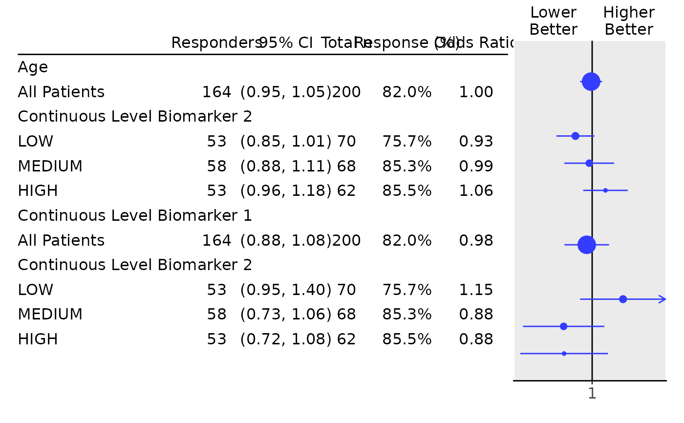
tabulate_rsp_biomarkers(df)
#>                                  Total n   Responders   Response (%)   Odds Ratio      95% CI      p-value (Wald)
#> —————————————————————————————————————————————————————————————————————————————————————————————————————————————————
#> Age                                                                                                              
#>   All Patients                     200        164          82.0%          1.00      (0.95, 1.05)       0.8530    
#>   Continuous Level Biomarker 2                                                                                   
#>     LOW                            70          53          75.7%          0.93      (0.85, 1.01)       0.0845    
#>     MEDIUM                         68          58          85.3%          0.99      (0.88, 1.11)       0.8190    
#>     HIGH                           62          53          85.5%          1.06      (0.96, 1.18)       0.2419    
#> Continuous Level Biomarker 1                                                                                     
#>   All Patients                     200        164          82.0%          0.98      (0.88, 1.08)       0.6353    
#>   Continuous Level Biomarker 2                                                                                   
#>     LOW                            70          53          75.7%          1.15      (0.95, 1.40)       0.1584    
#>     MEDIUM                         68          58          85.3%          0.88      (0.73, 1.06)       0.1700    
#>     HIGH                           62          53          85.5%          0.88      (0.72, 1.08)       0.2104    

## Table with a manually chosen set of columns: leave out "pval", reorder.
tab <- tabulate_rsp_biomarkers(
  df = df,
  vars = c("n_rsp", "ci", "n_tot", "prop", "or")
)

## Finally produce the forest plot.
g_forest(tab, xlim = c(0.7, 1.4))

# }