Helper function to prepare a KM layout

Usage

h_km_layout(
  data,
  g_el,
  title,
  footnotes,
  annot_at_risk = TRUE,
  annot_at_risk_title = TRUE
)

Arguments

data

(data.frame)
survival data as pre-processed by h_data_plot.

g_el

(list of gtable)
list as obtained by h_decompose_gg().

title

(string)
plot title.

footnotes

(string)
plot footnotes.

annot_at_risk

(flag)
compute and add the annotation table reporting the number of patient at risk matching the main grid of the Kaplan-Meier curve.

annot_at_risk_title

(flag)
whether the "Patients at Risk" title should be added above the annot_at_risk table. Has no effect if annot_at_risk is FALSE. Defaults to TRUE.

Value

A grid layout.

Details

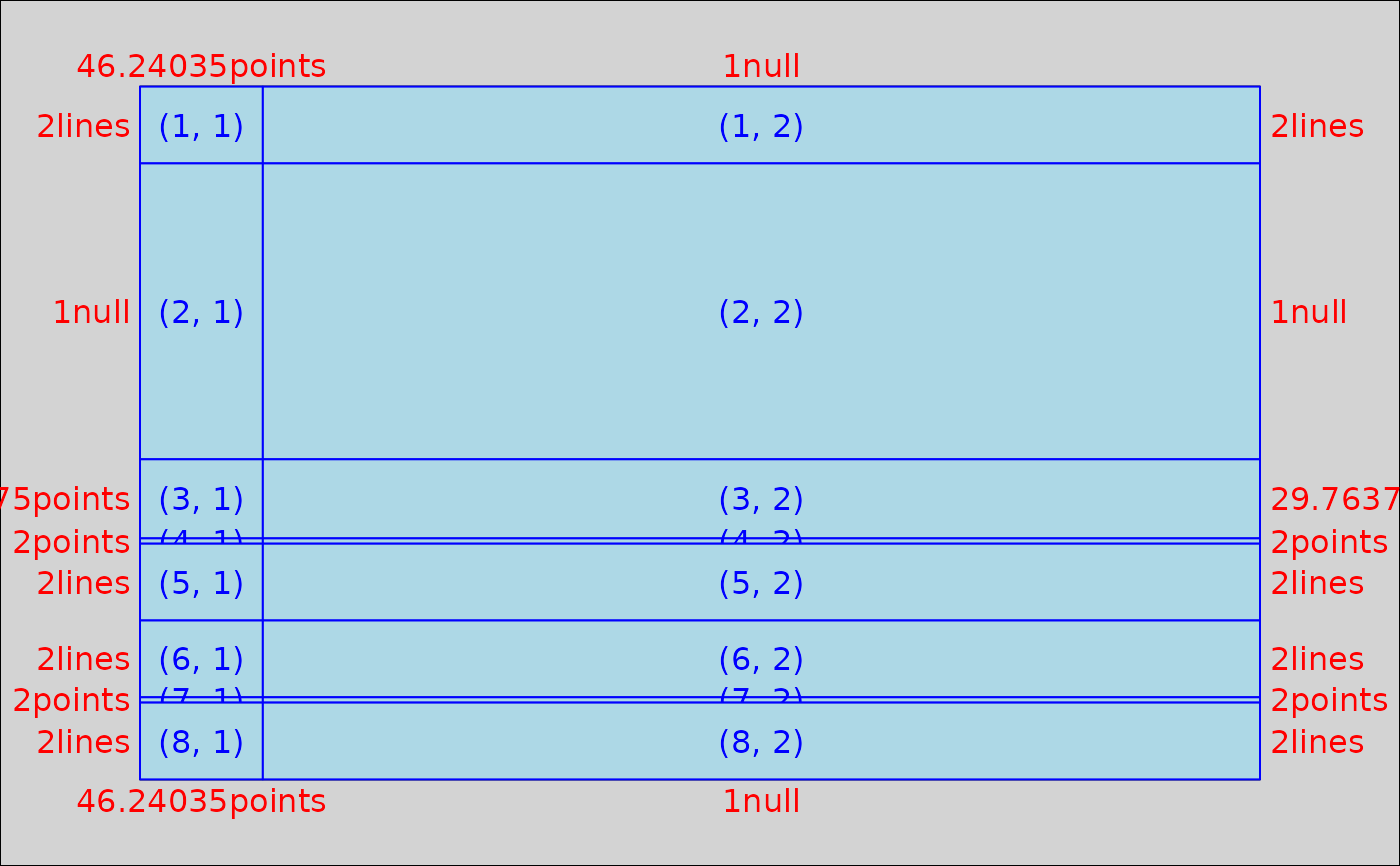
The layout corresponds to a grid of two columns and five rows of unequal dimensions. Most of the dimension are fixed, only the curve is flexible and will accommodate with the remaining free space.

• The left column gets the annotation of the ggplot (y-axis) and the names of the strata for the patient at risk tabulation. The main constraint is about the width of the columns which must allow the writing of the strata name.

• The right column receive the ggplot, the legend, the x-axis and the patient at risk table.

Examples

# \donttest{
library(dplyr)
library(survival)
library(grid)

fit_km <- tern_ex_adtte %>%
  filter(PARAMCD == "OS") %>%
  survfit(formula = Surv(AVAL, 1 - CNSR) ~ ARMCD, data = .)
data_plot <- h_data_plot(fit_km = fit_km)
xticks <- h_xticks(data = data_plot)
gg <- h_ggkm(
  data = data_plot,
  censor_show = TRUE,
  xticks = xticks, xlab = "Days", ylab = "Survival Probability",
  title = "tt", footnotes = "ff", yval = "Survival"
)
g_el <- h_decompose_gg(gg)
lyt <- h_km_layout(data = data_plot, g_el = g_el, title = "t", footnotes = "f")
grid.show.layout(lyt)

# }