Kaplan-Meier Plot — g

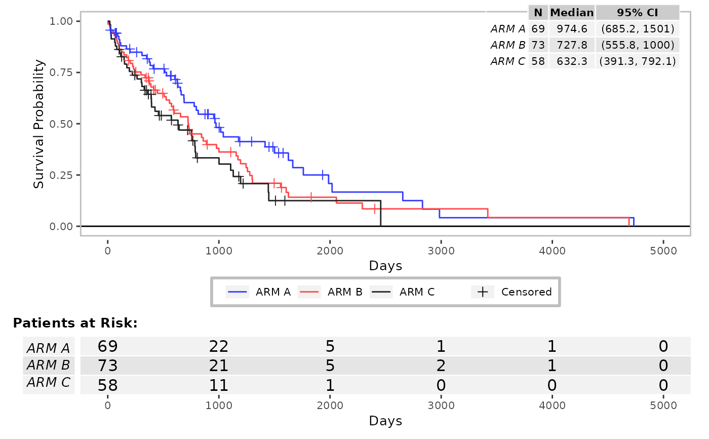
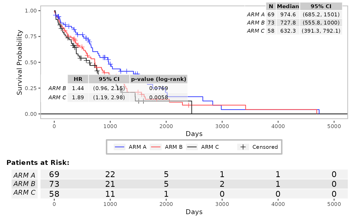
From a survival model, a graphic is rendered along with tabulated annotation including the number of patient at risk at given time and the median survival per group.

Usage

g_km(
  df,
  variables,
  control_surv = control_surv_timepoint(),
  col = NULL,
  lty = NULL,
  lwd = 0.5,
  censor_show = TRUE,
  pch = 3,
  size = 2,
  max_time = NULL,
  xticks = NULL,
  xlab = "Days",
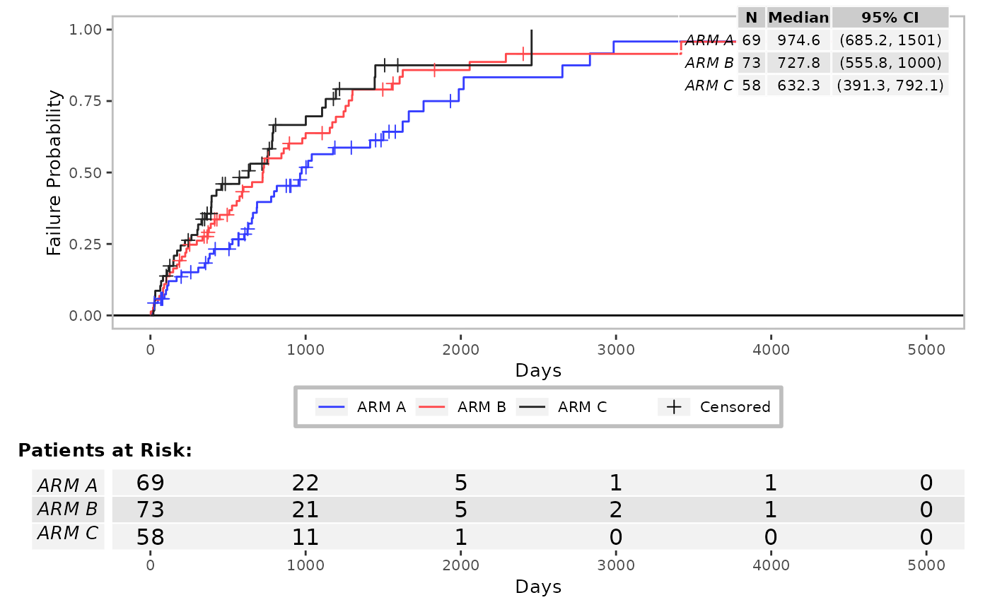
  yval = c("Survival", "Failure"),
  ylab = paste(yval, "Probability"),
  ylim = NULL,
  title = NULL,
  footnotes = NULL,
  draw = TRUE,
  newpage = TRUE,
  gp = NULL,
  vp = NULL,
  name = NULL,
  font_size = 12,
  ci_ribbon = FALSE,
  ggtheme = nestcolor::theme_nest(),
  annot_at_risk = TRUE,
  annot_at_risk_title = TRUE,
  annot_surv_med = TRUE,
  annot_coxph = FALSE,
  annot_stats = NULL,
  annot_stats_vlines = FALSE,
  control_coxph_pw = control_coxph(),
  position_coxph = c(-0.03, -0.02),
  position_surv_med = c(0.95, 0.9),
  width_annots = list(surv_med = grid::unit(0.3, "npc"), coxph = grid::unit(0.4, "npc"))
)

Arguments

df

(data.frame)
data set containing all analysis variables.

variables

(named list)
variable names. Details are:

tte (numeric)
variable indicating time-to-event duration values.
is_event (logical)
event variable. TRUE if event, FALSE if time to event is censored.
arm (factor)
the treatment group variable.
strat (character or NULL)
variable names indicating stratification factors.

control_surv

(list)
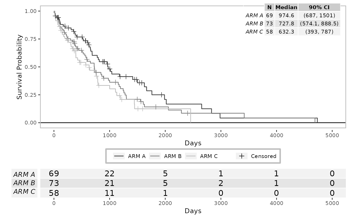
parameters for comparison details, specified by using the helper function control_surv_timepoint(). Some possible parameter options are:

conf_level (proportion)
confidence level of the interval for survival rate.
conf_type (string)
"plain" (default), "log", "log-log" for confidence interval type, see more in survival::survfit(). Note that the option "none" is no longer supported.

col

(character)
lines colors. Length of a vector should be equal to number of strata from survival::survfit().

lty

(numeric)
line type. Length of a vector should be equal to number of strata from survival::survfit().

lwd

(numeric)
line width. Length of a vector should be equal to number of strata from survival::survfit().

censor_show

(flag)
whether to show censored.

pch

(numeric, string)
value or character of points symbol to indicate censored cases.

size

(numeric)
size of censored point, a class of unit.

max_time

(numeric)
maximum value to show on X axis. Only data values less than or up to this threshold value will be plotted (defaults to NULL).

xticks

(numeric, number, or NULL)
numeric vector of ticks or single number with spacing between ticks on the x axis. If NULL (default), labeling::extended() is used to determine an optimal tick position on the x axis.

xlab

(string)
label of x-axis.

yval

(string)
value of y-axis. Options are Survival (default) and Failure probability.

ylab

(string)
label of y-axis.

ylim

(vector of numeric)
vector of length 2 containing lower and upper limits for the y-axis. If NULL (default), the minimum and maximum y-values displayed are used as limits.

title

(string)
title for plot.

footnotes

(string)
footnotes for plot.

draw

(flag)
whether the plot should be drawn.

newpage

(flag)
whether the plot should be drawn on a new page. Only considered if draw = TRUE is used.

gp

A "gpar" object, typically the output from a call to the function gpar. This is basically a list of graphical parameter settings.

vp

a viewport object (or NULL).

name

a character identifier for the grob. Used to find the grob on the display list and/or as a child of another grob.

font_size

(number)
font size to be used.

ci_ribbon

(flag)
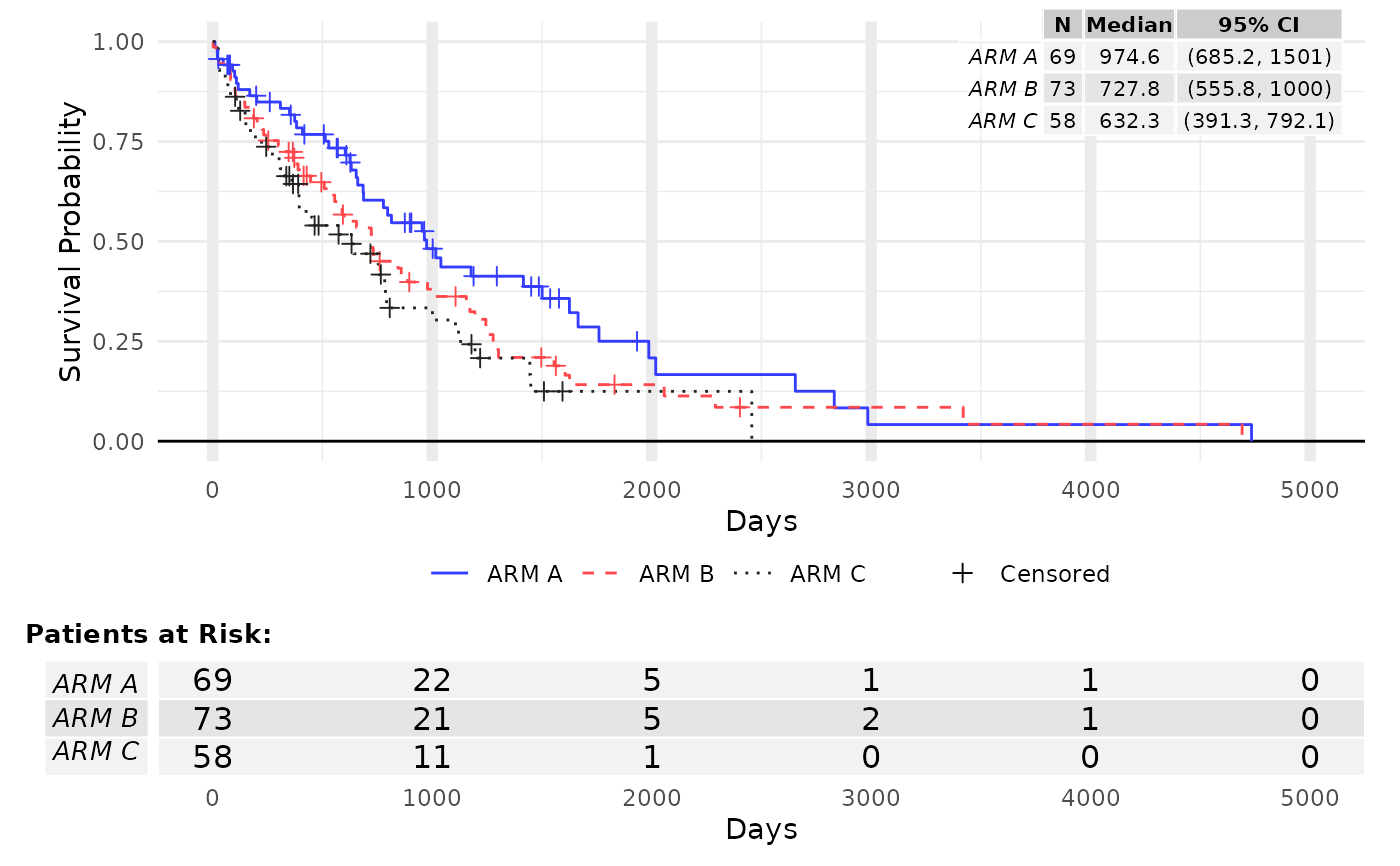
draw the confidence interval around the Kaplan-Meier curve.

ggtheme

(theme)
a graphical theme as provided by ggplot2 to control outlook of the Kaplan-Meier curve.

annot_at_risk

(flag)
compute and add the annotation table reporting the number of patient at risk matching the main grid of the Kaplan-Meier curve.

annot_at_risk_title

(flag)
whether the "Patients at Risk" title should be added above the annot_at_risk table. Has no effect if annot_at_risk is FALSE. Defaults to TRUE.

annot_surv_med

(flag)
compute and add the annotation table on the Kaplan-Meier curve estimating the median survival time per group.

annot_coxph

(flag)
add the annotation table from a survival::coxph() model.

annot_stats

(string)
statistics annotations to add to the plot. Options are median (median survival follow-up time) and min (minimum survival follow-up time).

annot_stats_vlines

(flag)
add vertical lines corresponding to each of the statistics specified by annot_stats. If annot_stats is NULL no lines will be added.

control_coxph_pw

(list)
parameters for comparison details, specified by using the helper function control_coxph(). Some possible parameter options are:

pval_method (string)
p-value method for testing hazard ratio = 1. Default method is "log-rank", can also be set to "wald" or "likelihood".
ties (string)
method for tie handling. Default is "efron", can also be set to "breslow" or "exact". See more in survival::coxph()
conf_level (proportion)
confidence level of the interval for HR.

position_coxph

(numeric)
x and y positions for plotting survival::coxph() model.

position_surv_med

(numeric)
x and y positions for plotting annotation table estimating median survival time per group.

width_annots

(named list of units)
a named list of widths for annotation tables with names surv_med (median survival time table) and coxph (survival::coxph() model table), where each value is the width (in units) to implement when printing the annotation table.

Value

A grob of class gTree.

Examples

# \donttest{
library(dplyr)
library(ggplot2)
library(survival)
library(grid)
library(nestcolor)

df <- tern_ex_adtte %>%
  filter(PARAMCD == "OS") %>%
  mutate(is_event = CNSR == 0)
variables <- list(tte = "AVAL", is_event = "is_event", arm = "ARMCD")

# 1. Example - basic option

res <- g_km(df = df, variables = variables)

res <- g_km(df = df, variables = variables, yval = "Failure")

res <- g_km(
  df = df,
  variables = variables,
  control_surv = control_surv_timepoint(conf_level = 0.9),
  col = c("grey25", "grey50", "grey75"),
  annot_at_risk_title = FALSE
)

res <- g_km(df = df, variables = variables, ggtheme = theme_minimal())

res <- g_km(df = df, variables = variables, ggtheme = theme_minimal(), lty = 1:3)

res <- g_km(df = df, variables = variables, max = 2000)

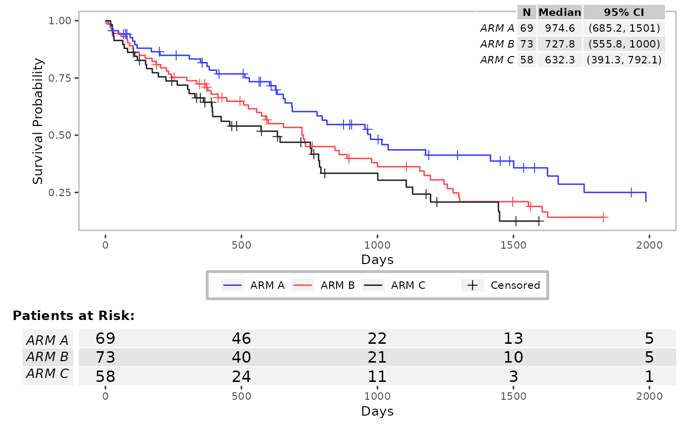res <- g_km(
  df = df,
  variables = variables,
  annot_stats = c("min", "median"),
  annot_stats_vlines = TRUE
)


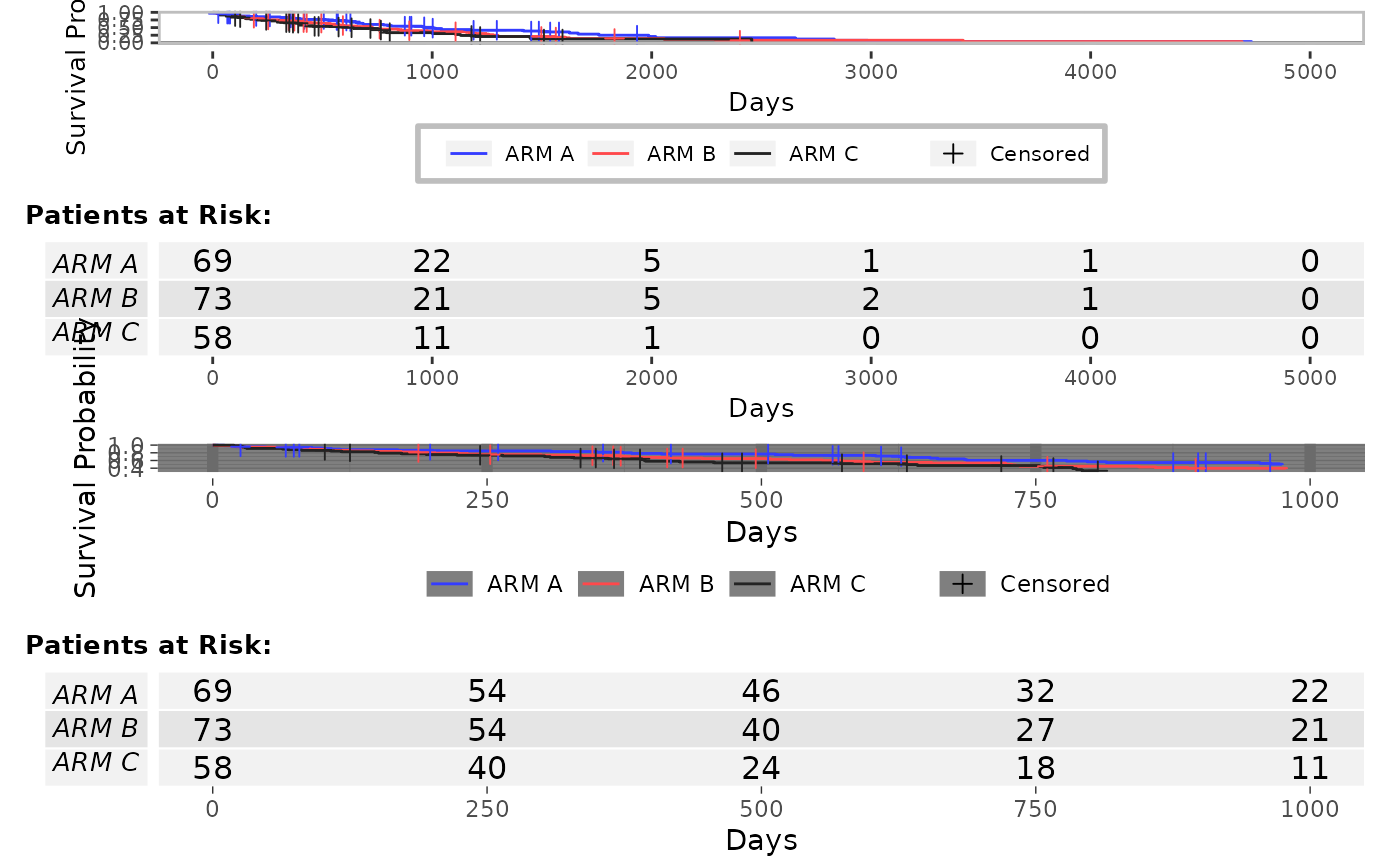
# 2. Example - Arrange several KM curve on a single graph device

# 2.1 Use case: A general graph on the top, a zoom on the bottom.
grid.newpage()
lyt <- grid.layout(nrow = 2, ncol = 1) %>%
  viewport(layout = .) %>%
  pushViewport()

res <- g_km(
  df = df, variables = variables, newpage = FALSE, annot_surv_med = FALSE,
  vp = viewport(layout.pos.row = 1, layout.pos.col = 1)
)
res <- g_km(
  df = df, variables = variables, max = 1000, newpage = FALSE, annot_surv_med = FALSE,
  ggtheme = theme_dark(),
  vp = viewport(layout.pos.row = 2, layout.pos.col = 1)
)


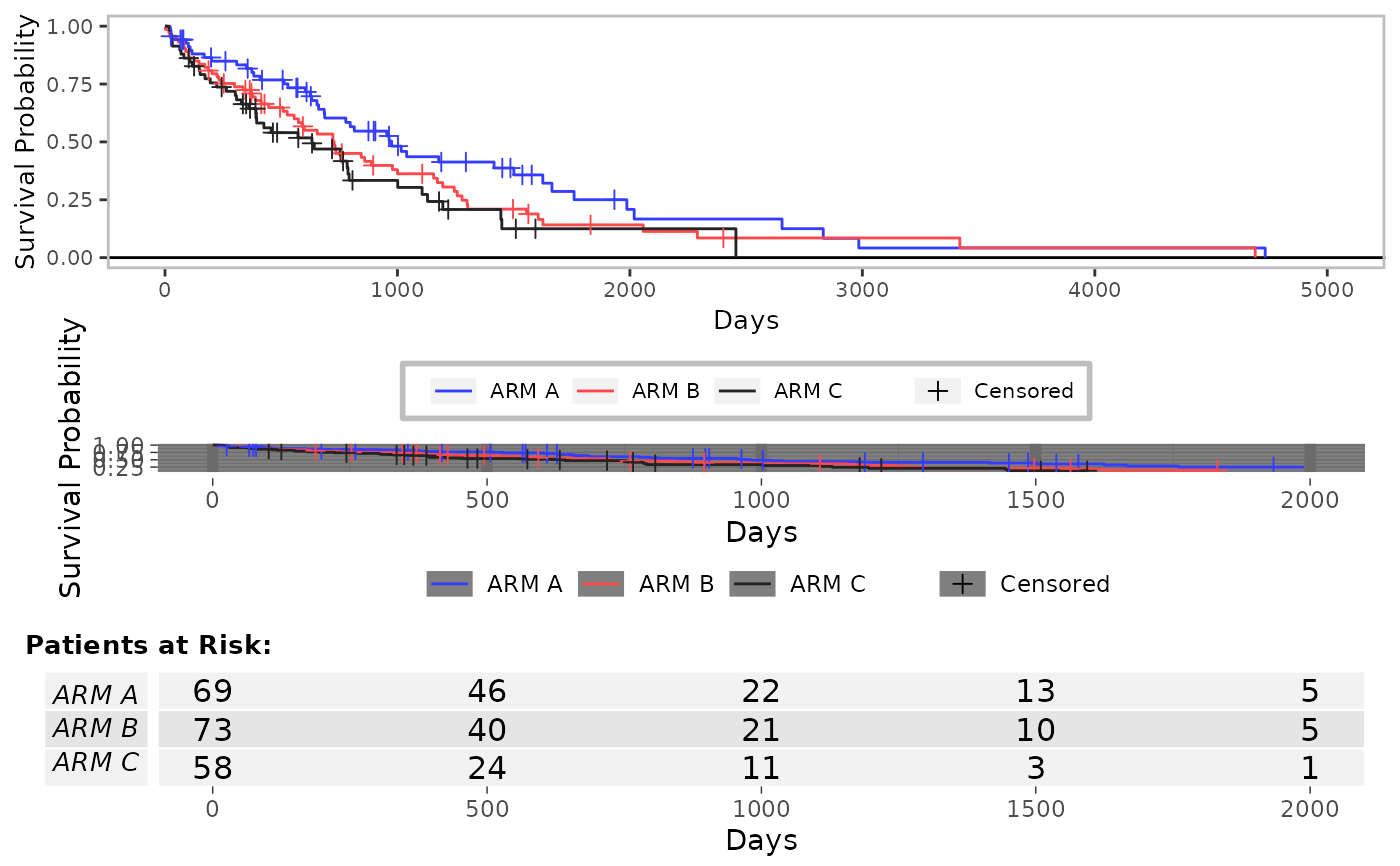
# 2.1 Use case: No annotations on top, annotated graph on bottom
grid.newpage()
lyt <- grid.layout(nrow = 2, ncol = 1) %>%
  viewport(layout = .) %>%
  pushViewport()

res <- g_km(
  df = df, variables = variables, newpage = FALSE,
  annot_surv_med = FALSE, annot_at_risk = FALSE,
  vp = viewport(layout.pos.row = 1, layout.pos.col = 1)
)
res <- g_km(
  df = df, variables = variables, max = 2000, newpage = FALSE, annot_surv_med = FALSE,
  annot_at_risk = TRUE,
  ggtheme = theme_dark(),
  vp = viewport(layout.pos.row = 2, layout.pos.col = 1)
)


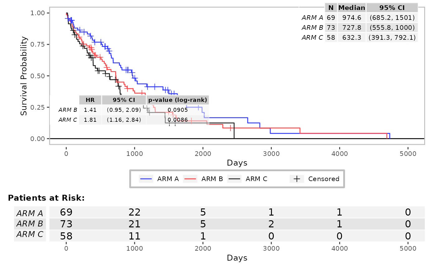
# Add annotation from a pairwise coxph analysis
g_km(
  df = df, variables = variables,
  annot_coxph = TRUE
)


# Change widths/sizes of surv_med and coxph annotation tables.
g_km(
  df = df, variables = c(variables, list(strat = "SEX")),
  annot_coxph = TRUE,
  width_annots = list(surv_med = grid::unit(2, "in"), coxph = grid::unit(3, "in"))
)


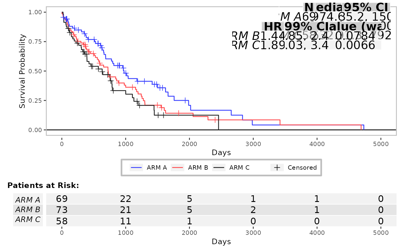
g_km(
  df = df, variables = c(variables, list(strat = "SEX")),
  font_size = 15,
  annot_coxph = TRUE,
  control_coxph = control_coxph(pval_method = "wald", ties = "exact", conf_level = 0.99),
  position_coxph = c(0.5, 0.5)
)


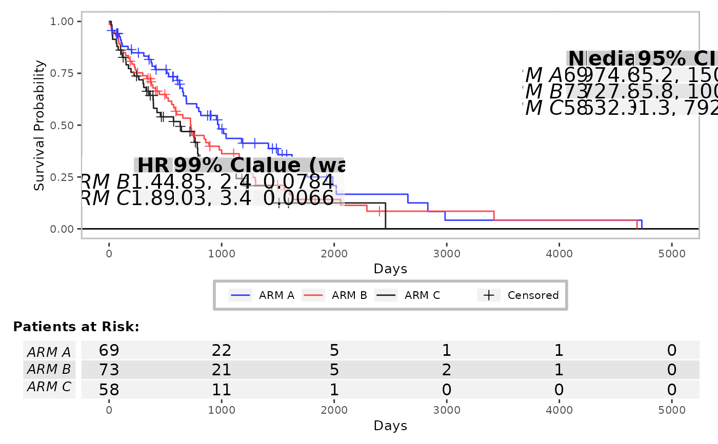
# Change position of the treatment group annotation table.
g_km(
  df = df, variables = c(variables, list(strat = "SEX")),
  font_size = 15,
  annot_coxph = TRUE,
  control_coxph = control_coxph(pval_method = "wald", ties = "exact", conf_level = 0.99),
  position_surv_med = c(1, 0.7)
)

# }