Create a Forest Plot based on a Table

Usage

g_forest(
  tbl,
  col_x = attr(tbl, "col_x"),
  col_ci = attr(tbl, "col_ci"),
  vline = 1,
  forest_header = attr(tbl, "forest_header"),
  xlim = c(0.1, 10),
  logx = TRUE,
  x_at = c(0.1, 1, 10),
  width_row_names = NULL,
  width_columns = NULL,
  width_forest = grid::unit(1, "null"),
  col_symbol_size = attr(tbl, "col_symbol_size"),
  col = getOption("ggplot2.discrete.colour")[1],
  draw = TRUE,
  newpage = TRUE
)

Arguments

tbl: (rtable)
col_x: (integer)
column index with estimator. By default tries to get this from tbl attribute col_x, otherwise needs to be manually specified.
col_ci: (integer)
column index with confidence intervals. By default tries to get this from tbl attribute col_ci, otherwise needs to be manually specified.
vline: (number)
x coordinate for vertical line, if NULL then the line is omitted.
forest_header: (character, length 2)
text displayed to the left and right of vline, respectively. If vline = NULL then forest_header needs to be NULL too. By default tries to get this from tbl attribute forest_header.
xlim: (numeric)
limits for x axis.
logx: (flag)
show the x-values on logarithm scale.
x_at: (numeric)
x-tick locations, if NULL they get automatically chosen.
width_row_names: (unit)
width for row names. If NULL the widths get automatically calculated. See grid::unit().
width_columns: (unit)
widths for the table columns. If NULL the widths get automatically calculated. See grid::unit().
width_forest: (unit)
width for the forest column. If NULL the widths get automatically calculated. See grid::unit().
col_symbol_size: (integer)
column index from tbl containing data to be used to determine relative size for estimator plot symbol. Typically, the symbol size is proportional to the sample size used to calculate the estimator. If NULL, the same symbol size is used for all subgroups. By default tries to get this from tbl attribute col_symbol_size, otherwise needs to be manually specified.
col: (character)
color(s).
draw: (flag)
whether the plot should be drawn.
newpage: (flag)
whether the plot should be drawn on a new page. Only considered if draw = TRUE is used.

Value

gTree object containing the forest plot and table.

Details

Create a forest plot from any rtables::rtable() object that has a column with a single value and a column with 2 values.

Examples

# \donttest{
library(dplyr)
library(forcats)
library(nestcolor)

adrs <- tern_ex_adrs
n_records <- 20
adrs_labels <- formatters::var_labels(adrs, fill = TRUE)
adrs <- adrs %>%
  filter(PARAMCD == "BESRSPI") %>%
  filter(ARM %in% c("A: Drug X", "B: Placebo")) %>%
  slice(seq_len(n_records)) %>%
  droplevels() %>%
  mutate(
    # Reorder levels of factor to make the placebo group the reference arm.
    ARM = fct_relevel(ARM, "B: Placebo"),
    rsp = AVALC == "CR"
  )
formatters::var_labels(adrs) <- c(adrs_labels, "Response")
df <- extract_rsp_subgroups(
  variables = list(rsp = "rsp", arm = "ARM", subgroups = c("SEX", "STRATA2")),
  data = adrs
)
# Full commonly used response table.

tbl <- basic_table() %>%
  tabulate_rsp_subgroups(df)
p <- g_forest(tbl)

draw_grob(p)


# Odds ratio only table.

tbl_or <- basic_table() %>%
  tabulate_rsp_subgroups(df, vars = c("n_tot", "or", "ci"))
tbl_or
#> Baseline Risk Factors                                           
#>                           Total n   Odds Ratio       95% CI     
#> ————————————————————————————————————————————————————————————————
#> All Patients                20         0.76       (0.10, 5.96)  
#> Sex                                                             
#>   F                         11       >999.99     (0.00, >999.99)
#>   M                          9         0.22       (0.01, 3.98)  
#> Stratification Factor 2                                         
#>   S1                        10         1.00       (0.05, 22.18) 
#>   S2                        10         0.67       (0.04, 11.29) 
p <- g_forest(
  tbl_or,
  forest_header = c("Comparison\nBetter", "Treatment\nBetter")
)

draw_grob(p)


# Survival forest plot example.
adtte <- tern_ex_adtte
# Save variable labels before data processing steps.
adtte_labels <- formatters::var_labels(adtte, fill = TRUE)
adtte_f <- adtte %>%
  filter(
    PARAMCD == "OS",
    ARM %in% c("B: Placebo", "A: Drug X"),
    SEX %in% c("M", "F")
  ) %>%
  mutate(
    # Reorder levels of ARM to display reference arm before treatment arm.
    ARM = droplevels(fct_relevel(ARM, "B: Placebo")),
    SEX = droplevels(SEX),
    AVALU = as.character(AVALU),
    is_event = CNSR == 0
  )
labels <- list(
  "ARM" = adtte_labels["ARM"],
  "SEX" = adtte_labels["SEX"],
  "AVALU" = adtte_labels["AVALU"],
  "is_event" = "Event Flag"
)
formatters::var_labels(adtte_f)[names(labels)] <- as.character(labels)
df <- extract_survival_subgroups(
  variables = list(
    tte = "AVAL",
    is_event = "is_event",
    arm = "ARM", subgroups = c("SEX", "BMRKR2")
  ),
  data = adtte_f
)
table_hr <- basic_table() %>%
  tabulate_survival_subgroups(df, time_unit = adtte_f$AVALU[1])
g_forest(table_hr)

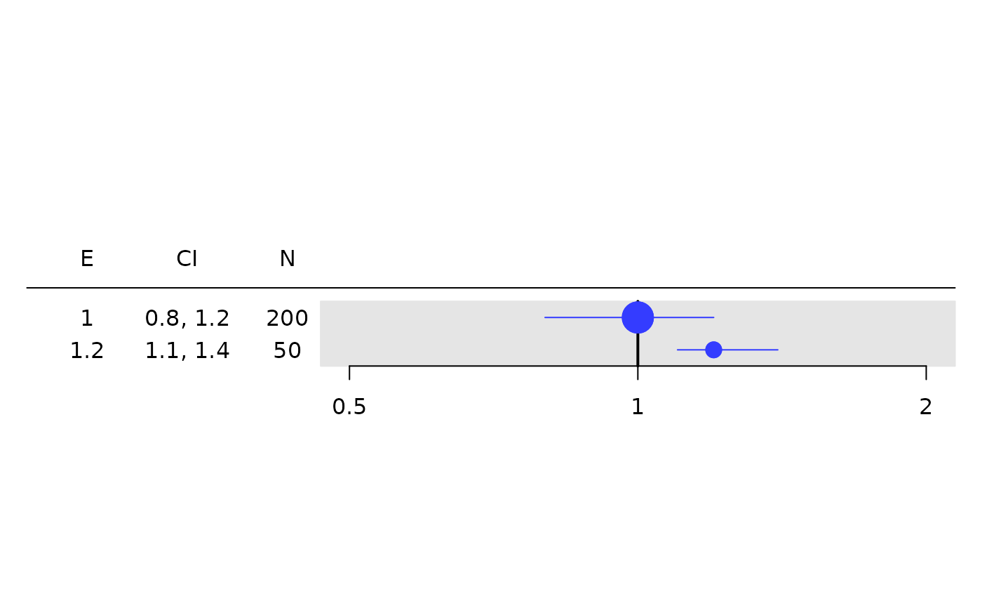
# Works with any `rtable`.
tbl <- rtable(
  header = c("E", "CI", "N"),
  rrow("", 1, c(.8, 1.2), 200),
  rrow("", 1.2, c(1.1, 1.4), 50)
)
g_forest(
  tbl = tbl,
  col_x = 1,
  col_ci = 2,
  xlim = c(0.5, 2),
  x_at = c(0.5, 1, 2),
  col_symbol_size = 3
)

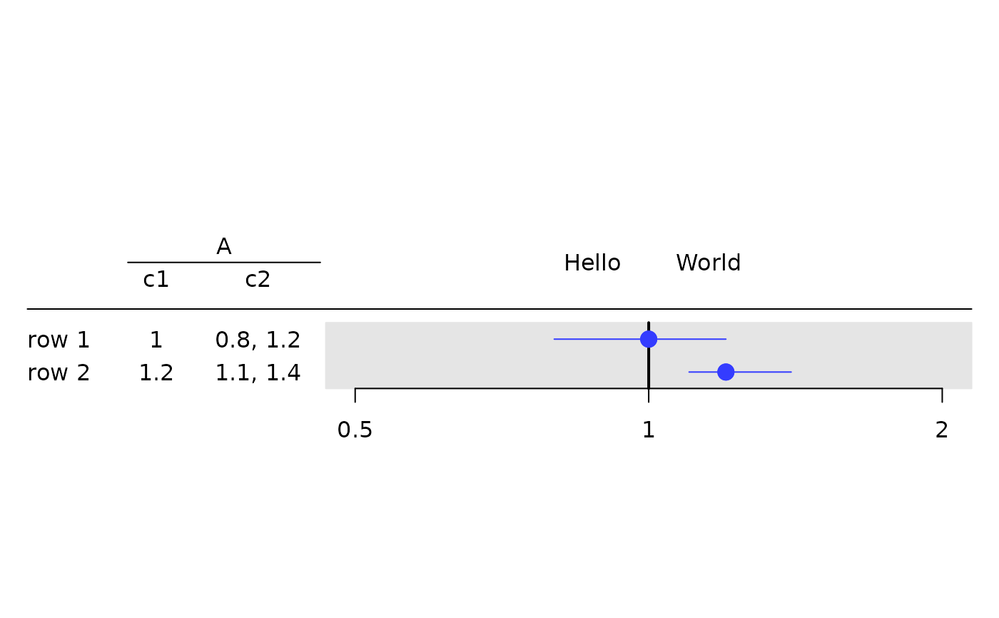
tbl <- rtable(
  header = rheader(
    rrow("", rcell("A", colspan = 2)),
    rrow("", "c1", "c2")
  ),
  rrow("row 1", 1, c(.8, 1.2)),
  rrow("row 2", 1.2, c(1.1, 1.4))
)
g_forest(
  tbl = tbl,
  col_x = 1,
  col_ci = 2,
  xlim = c(0.5, 2),
  x_at = c(0.5, 1, 2),
  vline = 1,
  forest_header = c("Hello", "World")
)

# }